NOTE: This is not supposed to be a happy and easy track. You will likely achieve nothing else but learning how hard life is! If you don’t have a super awesome PC, you won’t be able to run training at all. Generation is a bit more forgiving.
Note: Get the code here https://github.com/cybercom-finland/hacking-great-3 using: git clone https://github.com/cybercom-finland/hacking-great-3.
Update the code in the event to get the latest changes using: git pull --rebase.
Download the corpus8k.wav to the corpus directory. You only need it if you want to try training the network.
Note that training the network takes weeks, but you can try it anyhow. Note: Name the corpus8k.wav as corpus.wav
for the process.py to find it.
The pre-trained model was trained on 48 kHz corpus. The sound model is snapshotted to files sound-model and sound-model.meta.
The sample rate of the corpus makes little difference to the model (no, not even in terms of memory required), but smaller sample rate makes learning a bit faster. You only need to understand that the output of the model is in the same sample rate also.
If you want the better quality corpus, in 48k sample rate, there is corpus.wav also. Note that training that requires several months. It’s also quite large, almost 1 GB.
The corpus directory contains two files (after you downloaded the corpus.wav):
corpus8k.wav: approximately 1.5 hours of Communist music concatenated to a single channel 8 kHz WAV file.test8k.wav: A Communist music piece not included in the corpus for use as a test example.Validation set is skipped, as the real validation happens in generating sounds with the system.

The model used is a WaveNet with a receptive field size of 4093 samples. In 48 kHz wave it corresponds to 0.085 seconds of audio. It has a stack of four ten-layer exponential (1, 2, 4, 8, …, 512) stride atrous convolutional layers.
Training such large models will take 1-2 months using decent consumer grade hardware. Because of this, we weren’t able to have a very well trained final model, but we will have some model that probably leans towards Leninism a bit even though it is not yet completely brainwashed yet.
Joking aside, the technical side in training these models is that the model learns a decent prediction model pretty fast and gets decent loss values and 1-step forward outputs for training inputs. However, the network has a lot of uncertainty at occasional situations leading to snapping sounds in generation. That is because the model output gives a somewhat uniform distribution of amplitude values when uncertain. Sometimes these lead to snaps when in generation a somewhat improbable outlier is selected.
Additionally in generation is is important that the model has totally saturated its internal representation probability distributions so that it does not have large volumes of value space dedicated to situations that do not match training data. This is because in generation the uncertainty accumulates quickly, and a small divergence in the generated output that is not exactly something seen in the training data is not generalized well by the model when fed back to the input, causing internal representations in non-training space volume, and this causes noise in the output, because the output neurons haven’t seen such internal representations in training and their respective output is pretty much undefined. So, for not completely trained models the generated output is colored noise that has some amplitude envelope structure.
Deep learning is like pulled pork. You have to cook it for a long time.
After about 2 weeks of cooking (training) on an i5-4690 CPU @ 3.50GHz with 24 GB of memory (Note that the model is too large for any consumer grade GPU system) we got something like this: (temperature_temperaturedecimal_index).wav. Possibly before the event the quality is a bit better, but not much.
You can well skip this step, as it takes a really long time (months) to properly train this kind of model. But you can kind of try it out and see where it is going. Intermediate results are interesting to look at and play with also, even if they are very noisy. Not fully trained models cannot be used very effectively for generating waveforms, as the results are pretty much noise.
NOTE: Training takes a lot of memory, so for a normal laptop it is quite probable that swapping will occur and the machine freezes totally. It is recommended to turn off swap for such workloads. Regardless the training is so resource intensive that it will likely prevent all other use of the computer.
You can train a model using a command python process.py --model sound-model. The –model parameter is
optional, and specifies the starting point for training. Check also the parameters for the model
in the file params.py.
The repository will contain a pre-trained model, so you can skip this step.
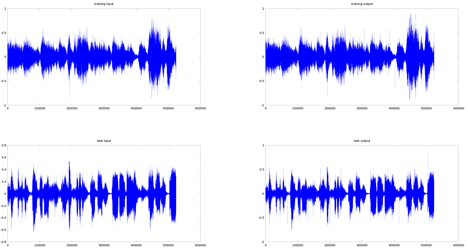
Training the model well (over 3 weeks on decent hardware) the results will look like something like this
plotting the resultant data in Octave
using the plot_training.m Octave script.

The trained model snapshots are stored to sound-model and sound-model.meta files. For convenience,
the model that achieved the best test accuracy against the test input/output pair is stored in the sound-model-best and sound-model-best.meta.
The waveforms are generated by feeding the trained model a seed wave. The system then tries to predict the next sample, or more accurately it predicts the discrete distribution in 256-valued µ-law encoding for the next sample. The system then picks a value from this predicted distribution, and it is added to the end of the seed wave. Then this is repeated, and the system generates a sound wave based on the initial seed.
This example uses trivial generation, processing the entire input again for the next sample. In practice, it is possible to optimize this greatly by using intermediate result from the previous prediction again for the next prediction. This is called “Fast WaveNet Generation Algorithm”, and is implemented for example in the other TensorFlow WaveNet implementation by ibab.
It takes a long time (several hours or so) to get reasonably long wave forms, but intermediate results can be interesting to look at.
You can generate a sound sample using a command python generate.py. Check also the parameters for the model
in the file params.py. Note that in generation the model related parameters need to be identical to the parameters of the trained model for the snapshot restoration to work. You can play with the temperature parameter freely.
The repository will contain a set of pre-generated waveforms for different seed signals and temperatures, so you can skip this step.
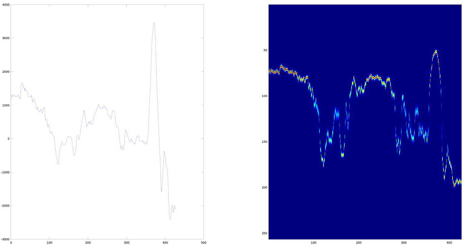
Generating a few steps of a sample will look like something like this plotting the resultant data in Octave
using the plot_generation.m Octave script.

You can also skip this step if you want and do other things. There are some generated example outputs in the samples directory for different values of temperature. For example filename 0_95.wav means a temperature
0.95 was used in the generation. 1_0_2.wavmeans this is the second example of generation using temperature of 1.0.
Temperature 1.0 means using the estimated probability distribution as is in the generation. Lower temperature means weighting the most likely options more, avoiding the less likely alternatives. Higher temperature means giving less weight for the most likely option, and weighting the less likely options more. The order of likelihood does not change between the options, only relative weighting.
All sound content belongs to their respective copyright holders. The concatenated WAV file is meant for academic research / teaching only on the basis of the respective copyright exceptions in the Finnish copyright law, American fair use and also noting that the property of a Communist is common.